Pareto Distribution in Python
Submitted by moazkhan on Tuesday, July 7, 2020 - 09:31.
In this tutorial you will learn:
- What is Pareto Distribution?
- Pareto Distribution Implementation in python
- Visualization of Pareto Distribution
Pareto Distribution
Pareto Distribution is a continuous power law distribution named after the famous 19th Century economist named Vilfredo Preto. Pareto Distribution is also known as Zipf distribution and as Riemann zeta distribution. It is commonly referred as Pareto Principle, “80-20” rule or Mathew Principle. An example for “80-20” rule could be the wealth distribution, that the 80% of wealth is held by 20% of the Italian population(statistics of 20th Century) .The pareto distribution can be used in variety of situations, as an example it could be used to model the life time of manufactured item with certain warranty period. Practical applications of Pareto Distribution includes business management, evaluation of company revenue sources, employee evaluation etc.Pareto Distribution in Python
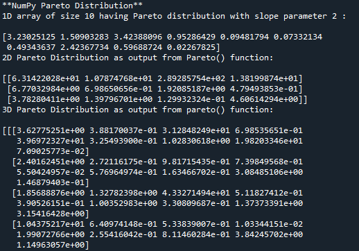
The random module of python’s NumPy library provide an inbuilt function pareto() for implementation of Pareto Distribution. The pareto() function takes in two mandatory parameters, first parameter is the “size” of the array which we require as an output.The second parameter “a” is the shape perimeter called as slope parameter or pareto index. The value of shape perimeter could be an unsigned float or int only. In order to enhance the understanding of Pareto Distribution, lets take an example. We will generate a 1D array(10,) of Pareto distribution with shape perimeter 2. In this code we can see that we are importing the random module in the second line of the code and in the fourth line we are applying the Pareto distribution with output size parameter (10,) and shape parameter ‘a’ equal to 2.- #importing the random module
- from numpy import random
- #applying the Pareto function
- res_arr= random.pareto(size=10,a=2.0)
- #printing the results
- print('1D array of size 10 having Pareto distribution with slope parameter 2 :\n')
- print(res_arr)
- #importing the random module
- from numpy import random
- #here we are using Pareto function to generate Pareto distribution of size 3 x 4 with shape parameter 0.5
- res_arr = random.pareto(size=(3,4),a=0.5)
- print('2D Pareto Distribution as output from Pareto() function:\n')
- #printing the result
- print(res_arr)
- #importing the random module
- from numpy import random
- #here we are using Pareto function to generate Pareto distribution of size 7 x 8 x 9
- res = random.pareto(size=(7,8,9), a=1)
- print('3D Pareto Distribution as output from pareto() function:\n')
- #printing the result
- print(res)
Visualization of Pareto Distribution
In this example we will visualize the Pareto Distribution with slope parameter 1.5. Here we will be using the displot function of seaborn library to plot and visualize a two dimensional pareto distribution- #importing all the required modules and packages
- from numpy import random
- import matplotlib.pyplot as mpl
- import seaborn as sb
- #here we are using Pareto function to generate distributions of size (1000,2) with slope parameter 1.5
- sb.distplot(random.pareto(size=(1000,2),a=1.5), hist=False, label='Pareto Distribution')
- #plotting the graph
- mpl.show()