Normal (Gaussian) Distribution with Python

Submitted by moazkhan on Friday, June 26, 2020 - 11:56.

In this tutorial you will learn:

What is a Gaussian Distribution?
Gaussian Distribution Implementation in python

Gaussian Distribution

Gaussian Distribution also known as normal distribution is a probability distribution that is symmetric about the mean and it depicts that that the frequency of values near the mean is greater as compared to the values away from the mean. Gaussian distributions are symmetrical while all symmetrical distributions are not Gaussian distributions. Gaussian distribution is characterized by the value of mean equal to zero while the value of standard deviation is one. The graphical pattern of a gaussian distribution always appears as a bell curve.

Gaussian Distribution in Python

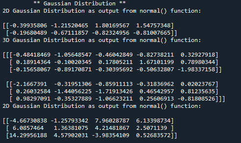
Gaussian distribution in python is implemented using normal() function. The normal() function is included in the random module. It takes in the “size” of the distribution which we want as an output as a first and mandatory parameter. It takes “loc” as a second parameter, the location determines the point of the peak. It take “scale” as a third parameter, the scale determines the how flat the graph distribution would be (also known as standard deviation). In this example we will generate a 2D array of normal distribution having size (2,4), in the first line of code we are importing random module from numpy library. In the third line of the code we are calling the normal() function with only mandatory parameter “size”.

from numpy import random
#here we are using normal function to generate gaussian distribution of size 2 x 4
res = random.normal(size=(2,4))
print('2D Gaussian Distribution as output from normal() function:\n')
#printing the result
print(res)

Lets take another example, in this example we will generate a 3D array of normal distribution of the size(2,4,5).

from numpy import random
#here we are using normal function to generate gaussian distribution of size 2 x 3 x 5
res = random.normal(size=(2,3,5))
print('3D Gaussian Distribution as output from normal() function:\n')
#printing the result
print(res)

In this example while calling the normal() function, we will also declare the standard deviation and location of the mean as 3 and 4 respectively. Here you can observe that I have given two additional parameters “size” and “loc” to normal() function.

from numpy import random
#here we are using normal function to generate gaussian distribution of size 3 x 4
res = random.normal(size=(3,4), loc= 3, scale = 4)
print('2D Gaussian Distribution as output from normal() function:\n')
#printing the result
print(res)

This is an important example, in this example we will visualize the array being generated by the normal() function with output array size 1000, standard deviation 4 and loc of mean 3. Here we will use the distplot() as used in last tutorial.

#importing all the required modules and packages
from numpy import random
import matplotlib.pyplot as mpl
import seaborn as sb
#here we are using normal function to generate gaussian distribution of size 1000
sb.distplot(random.normal(size=1000, loc = 3, scale = 4), hist=True)
#plotting the graph
mpl.show()

Add new comment

1319 views