Logistic Distribution in Python

In this tutorial you will learn:

• What is Logistic Distribution?
• Logistic Distribution Implementation in python
• Visualization of Logistic Distribution

Logistic Distribution

Logistic distribution is a continuous distribution used for modelling growth and logistic regression. Its graphical representation replicates the normal distribution, belongs to symmetrical family of distribution and always have one peak. It has really simple cumulative distribution formula due to which it replicates normal distribution extremely well. It is used in different areas such as physical sciences, sports modeling, financing, machine learning and neural networks.

Logistic Distribution in Python

Logistic distribution in python is implemented using an inbuilt function logistic() which is included in the random module of NumPy library. The logistic() function takes in one mandatory parameter and two optional parameters. First parameter “size” is the size of the output array which could be 1D, 2D, 3D or n-dimensional (depending on the programmer’s requirement). The second parameter is the standard deviation defined by “scale”, and if not explicitly defined, its value is taken as 1. Third parameter is the mean, it determines the location of peak and is defined by “loc”. If mean is not explicitly defined, it is taken as 0 by the logistic() function.
Lets take an example, we will generate a 1D array(1,4) of logistic distribution having mean at 3 with standard deviation of 1.5. Here you can observe that if we re run the program again and again, the values of the distribution will keep on changing.

#importing the random module
from numpy import random
#applying the logistic function with mean value 3 and standard deviation 1.5
res_arr= random.logistic(loc=3, scale=1.5, size=4)
#printing the results
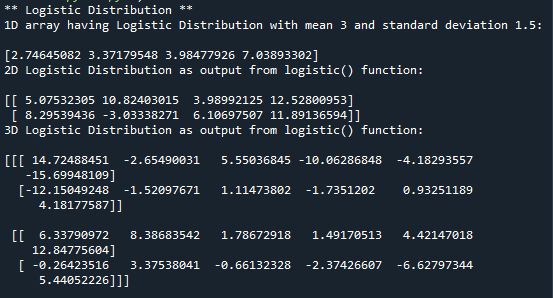
print('1D array having Logistic Distribution with mean 3 and standard deviation 1.5:/n')
print(res_arr)

#importing the random module
from numpy import random
#here we are using logistic function to generate rectangular distribution of size 2 x 4 with mean at 6 and standard deviation 3
res_arr = random.logistic(scale = 3, loc=6, size=(2,4))
print('2D Logistic Distribution as output from logistic() function:\n')
#printing the result
print(res_arr)

#importing the random module
from numpy import random
#here we are using logistic function to generate logistic distribution of size 2 x 2 x 6
res = random.logistic(size=(2,2,6), scale = 4, loc=2)
print('3D Logistic Distribution as output from logistic() function:\n')
#printing the result
print(res)

Visualization of Rectangular Distribution

In this example we will visualize the Logistic Distribution and Normal Distribution using the distplot() function, here we will be using the default values for both functions. Here we can observe that the plotted graphs appear almost identical. In order to clarify the differences, both graphs are plotted simultaneously.

#importing all the required modules and packages
from numpy import random
import matplotlib.pyplot as mpl
import seaborn as sb
#here we are using normal and logistic function to generate distributions of size 1000 with default parameters
sb.distplot(random.normal(size=1000), hist=False, label='normal')
sb.distplot(random.logistic(size=1000), hist=False, label='logistic')
#plotting the graph
mpl.show()